

System Dynamics | Foundation 9: One-Stock Systems Continued
The Drama Escalates

If you’ve ever tried to recover a language you once spoke fluently, stay with me until the end of this piece. By the time you finish, you’ll have a name for what happened, and it won’t be laziness.
In Foundation 8, we put two balancing loops on the same stock and watched them compete. Each loop had a goal. Each one sensed a discrepancy between that goal and the current state of the stock, and each one pushed corrective action in response. The drama came from the tug-of-war: which loop dominated, and by how much.
The structure we’re about to examine is different in a way that matters.
One of the two loops is still balancing. But the other is reinforcing, and a reinforcing loop doesn’t have a setpoint. It doesn’t sense discrepancy. It doesn’t correct toward anything. It simply amplifies whatever is already in the stock. More stock generates more inflow. Less stock generates less inflow. The loop feeds on itself.
This changes the character of the drama entirely. In a B+B system, there was at least an implicit promise of stability, two loops both trying to hold something. In an R+B system, there is no such promise. The stock can grow without bound, or it can collapse toward zero, depending entirely on which loop is stronger at any given moment.
This is one of the most common and consequential structures in the world. It describes every living population. It describes every economy. It describes how knowledge accumulates, and how it disappears.
Let’s look at it carefully.
The Population System
Consider a population. People born and people die. The stock is the number of people alive at any moment. It has one inflow: births. It has one outflow: deaths.
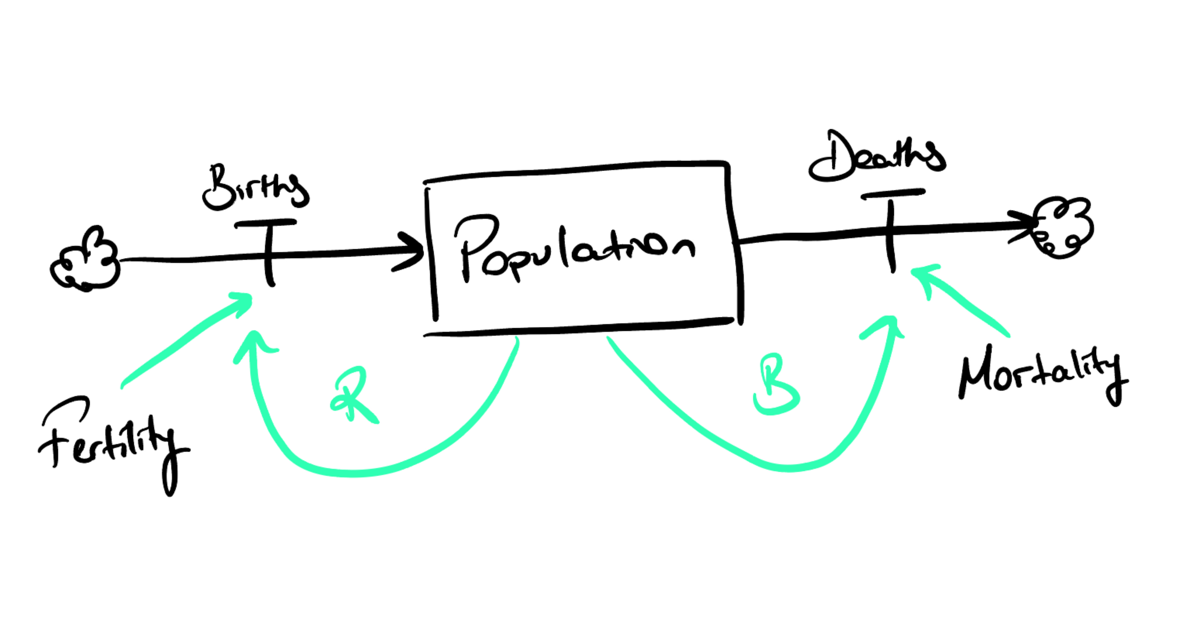
The birth loop is reinforcing. More people means more potential parents, which means more births, which means even more people. The loop is self-amplifying: the larger the population, the faster it grows, as long as fertility stays constant.
The death loop is balancing, but not in the way the thermostat was balancing. There is no goal state, no desired population level that the death loop is trying to restore. Deaths simply drain the stock at a rate proportional to how many people are in it. A larger population produces more deaths per year, which keeps the loop from being purely reinforcing, but the loop is not correcting toward anything. It is draining proportionally.
This distinction is subtle but important. The death loop doesn’t want the population to be smaller. It just removes a constant fraction of whatever is there.
The behavior of this system depends entirely on the relationship between the two loop strengths, that is, between the fertility rate and the mortality rate.
Three Behaviors
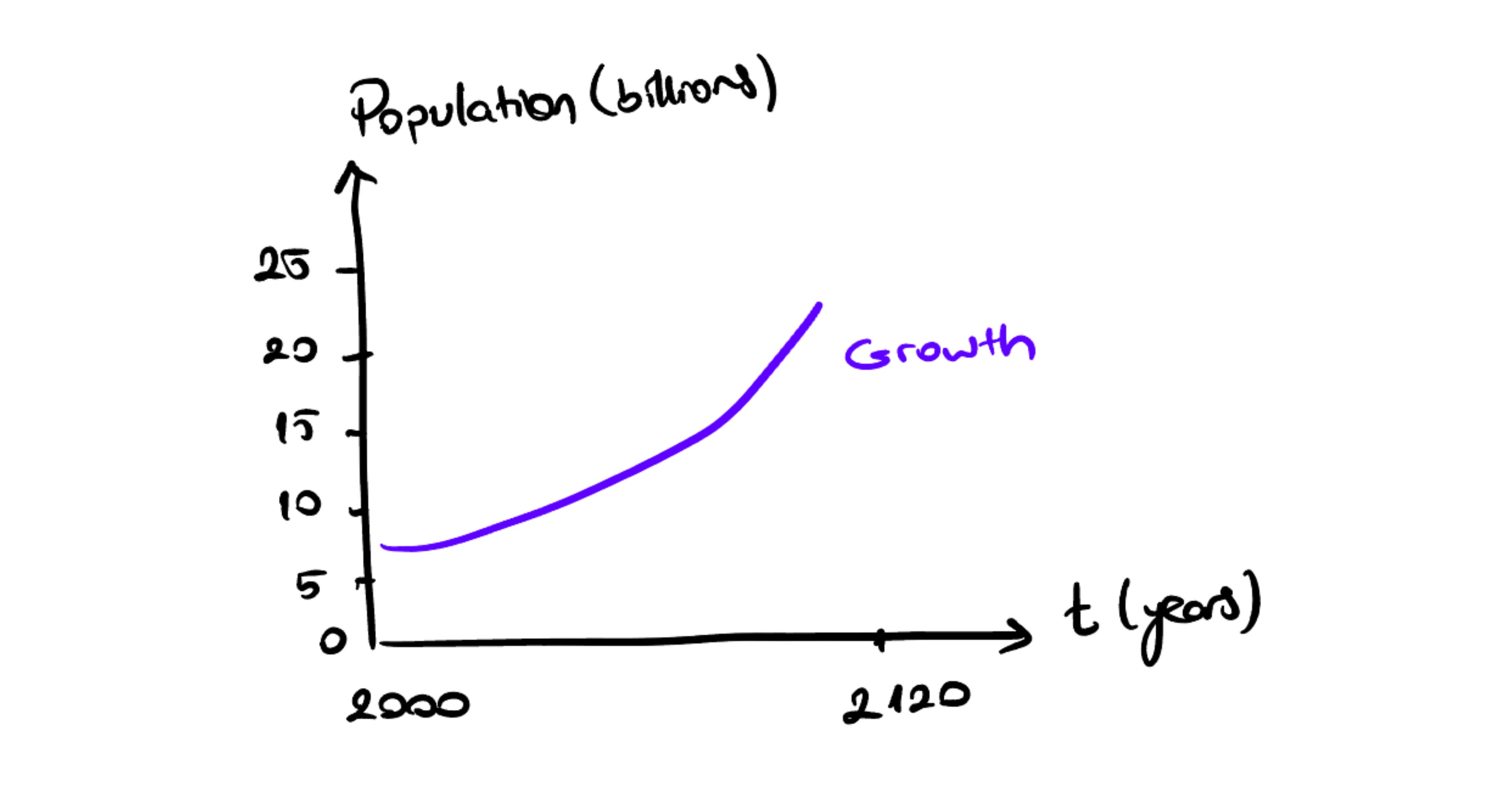
If fertility is higher than mortality, if the birth rate per thousand exceeds the death rate per thousand, the reinforcing loop dominates. The population grows, and it grows exponentially. Each year there are more people than the year before, and because there are more people, the following year brings even more births. The curve bends upward, accelerating.
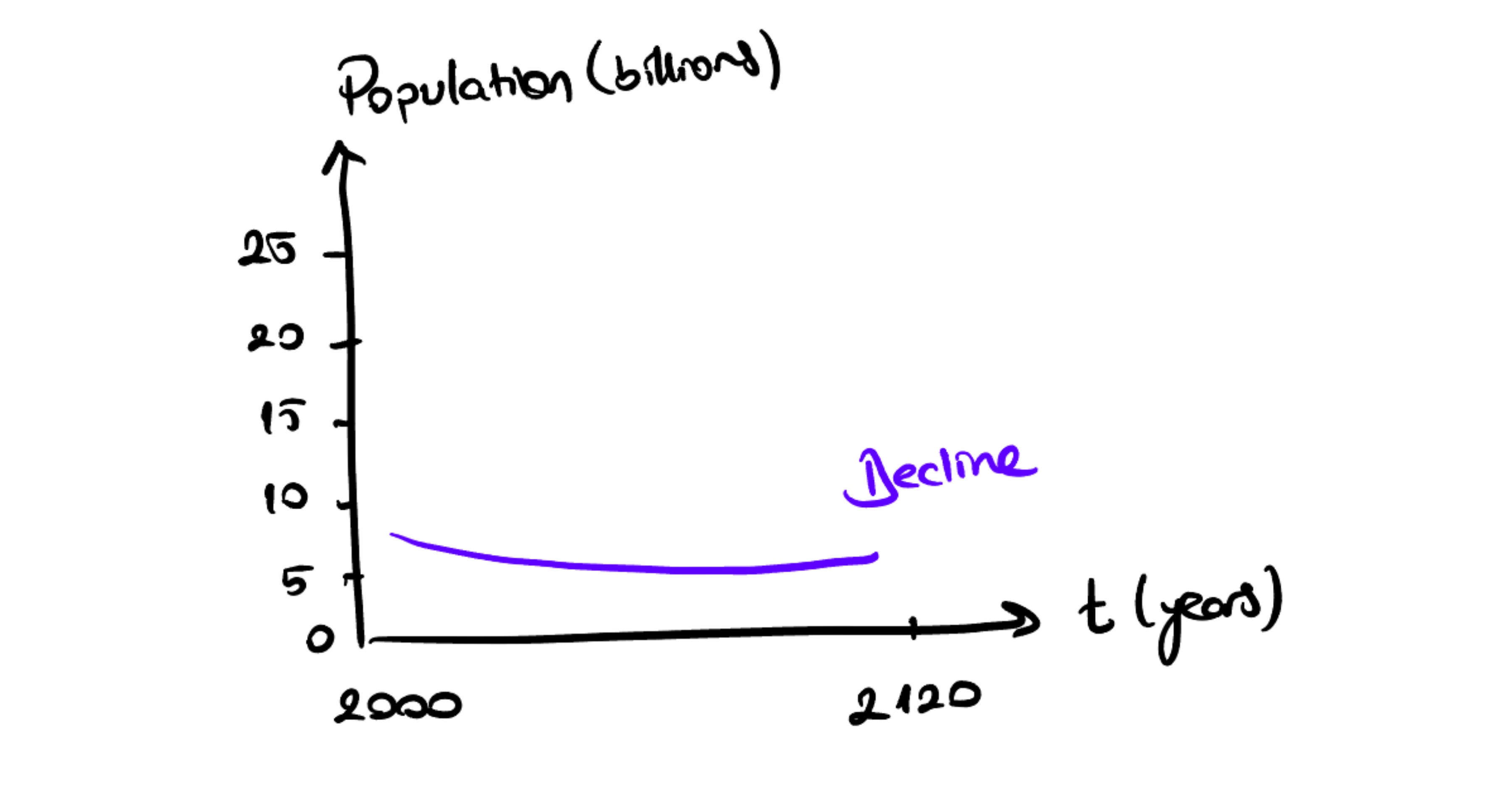
If mortality is higher than fertility, the balancing loop dominates. More people die each year than are born. The population declines. And because there are fewer people, the following year brings fewer births still. The reinforcing loop, now weak, no longer compensates for the drain. The curve bends downward, decelerating toward zero.
If fertility equals mortality exactly, the two loops are in balance. Births and deaths cancel out precisely. The population neither grows nor shrinks. This is dynamic equilibrium, the stock is stable, but it is stable because two active processes are exactly offsetting each other, not because nothing is happening.
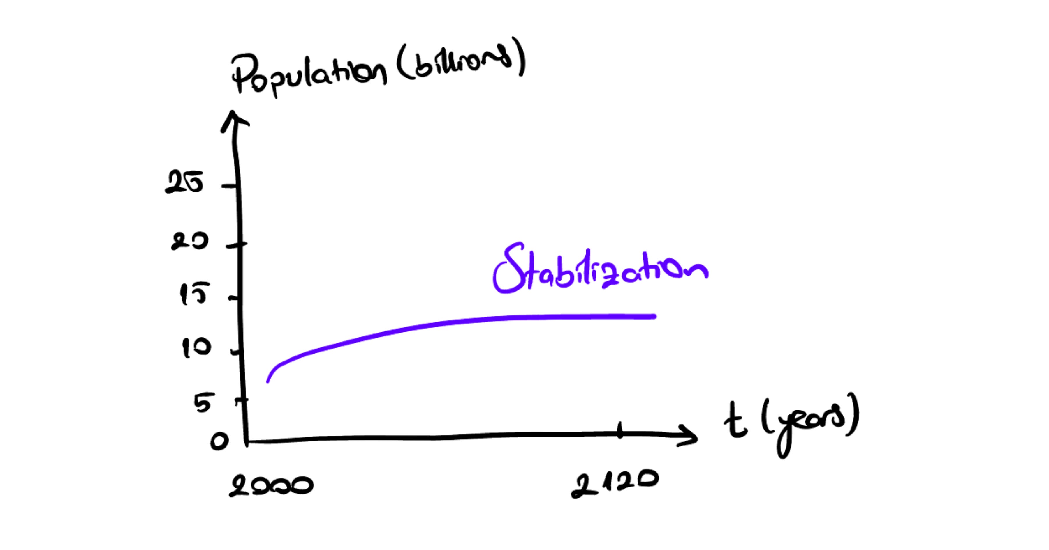
Three behaviors. Same structure. The only thing that changes is the ratio of loop strengths.
When Loop Strength Changes Over Time
The scenarios above assume fertility and mortality are constant. In real systems, they are not.
When the United Nations makes long-range population projections, it generally assumes that fertility will decline as countries develop, approaching replacement level, where on average each woman has just enough children to replace the current generation. It also assumes that mortality will continue to decline, though more slowly, as health care improves.
If fertility falls steadily over several decades and eventually equals mortality, the behavior curve doesn’t stay on one trajectory. It bends. Early on, with fertility well above mortality, the reinforcing loop dominates and population grows, but more slowly than it would under constant fertility. As fertility approaches mortality, the growth slows further. When they equalize, the curve flattens. The population stabilizes.
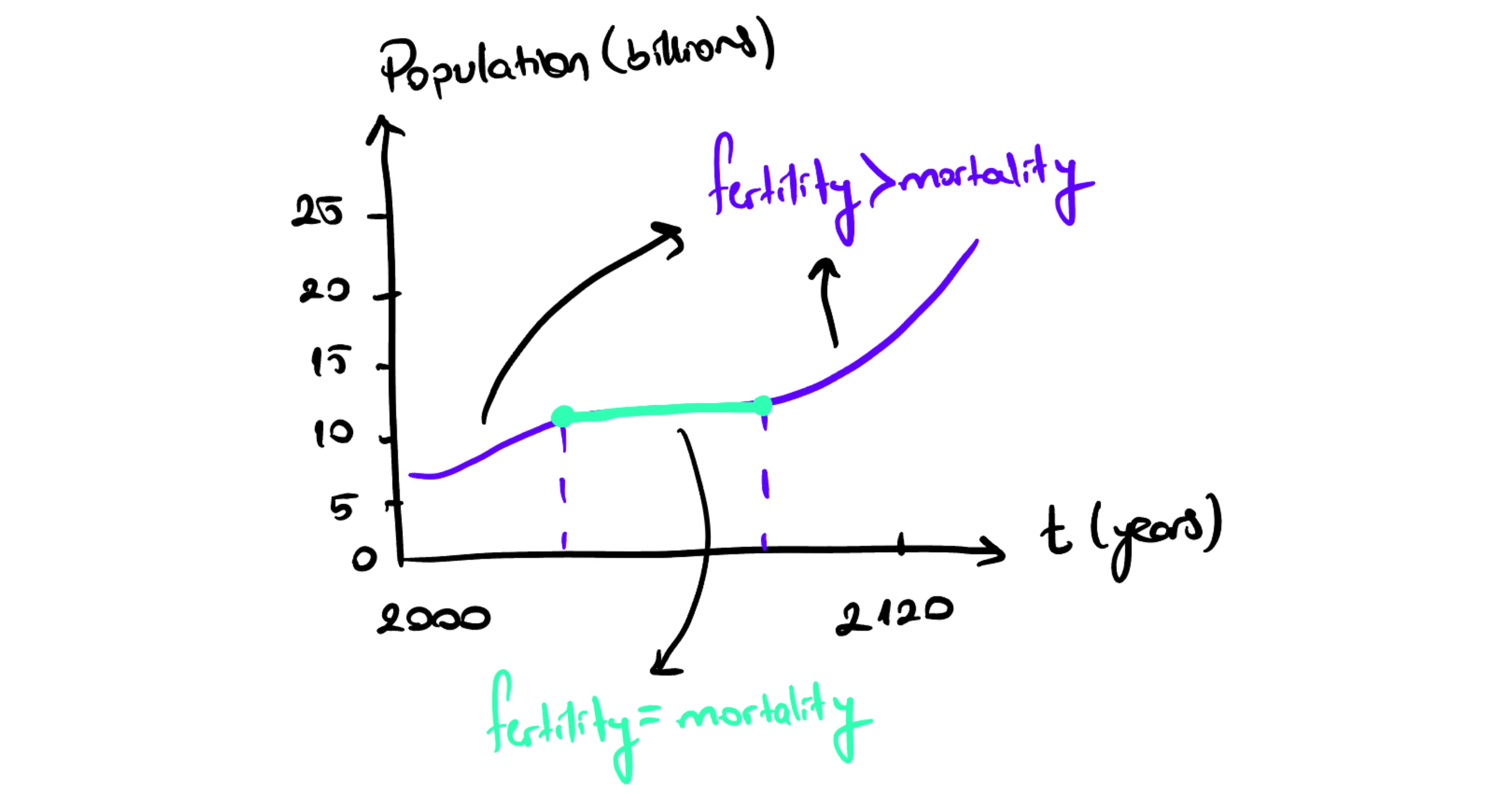
This is the signature of shifting dominance: the curve changes its character over time, because the relative strengths of the loops change over time. You are not looking at a single behavior mode. You are looking at a sequence of behavior modes, each produced by whichever loop is momentarily stronger.
Complex behaviors of systems often arise as the relative strengths of feedback loops shift, causing first one loop and then another to dominate behavior.
This will become important again shortly.
The Capital System
At the heart of every industrial economy is a structure that looks nothing like a population, and behaves exactly like one.
The stock is physical capital: machines, factories, infrastructure. It has one inflow: investment. It has one outflow: depreciation.
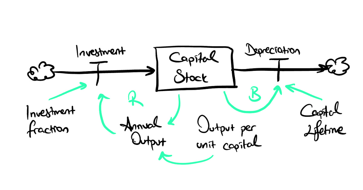
The investment loop is reinforcing. More capital produces more output. A fraction of that output is reinvested to create new capital. More capital → more output → more investment → more capital. The loop amplifies itself exactly as the birth loop does.
The depreciation loop is balancing, again, not toward a setpoint, but proportionally. Capital wears out, becomes obsolete, is retired. The fraction of the stock that depreciates each year depends on the average capital lifetime. A shorter lifetime means a higher annual depreciation rate. More capital means more absolute depreciation per year.
The structural isomorphism is exact:
Investment fraction = fertility
Capital lifetime = mortality analogue
Annual output per unit of capital = a parameter that scales the reinforcing loop’s strength
If the investment fraction is high enough relative to the depreciation rate, the reinforcing loop dominates: the capital stock grows exponentially. If the depreciation rate outpaces reinvestment, the stock declines. If they are matched, the economy is in dynamic equilibrium, producing enough each year to exactly replace what wears out, nothing more.
The same three behaviors. The same shifting dominance. A completely different system.
This is one of the central insights of systems theory.
Systems with similar feedback structures produce similar dynamic behaviors, regardless of how dissimilar they appear on the surface.
A factory is not a person. Depreciation is not death. But the feedback structure doesn’t care about appearances. It produces the same behavioral repertoire either way.
The Same Structure Where You Least Expected It
Consider two situations that feel nothing alike.
Second Language Fluency
You once spoke French. Or Spanish, or Mandarin whatever language you studied for years and then, somewhere in the years after, gradually stopped using. You probably describe what happened as forgetting. As letting it slip. As not keeping up with it.
Here is the structural description.
There is a reinforcing loop: competence enables successful communication, which builds confidence, which drives more frequent use, which builds more competence. This is why immersion works so quickly, the R loop runs at full strength, compounding daily. And there is a balancing loop: atrophy drains the stock at a rate proportional to its current size. The more you know, the more you can lose per year in absolute terms. The drain scales with the stock.
The loop structure here is real. The precise variables governing loop strength, how exactly confidence translates into use, how opportunity shapes the R loop’s reach, are harder to isolate than in population or capital. But the behavioral logic holds. When immersion ended, the conditions driving the R loop weakened. Use became infrequent, success less reliable, confidence fell further. The R loop dropped below the B loop. Dominance shifted. The curve bent from growth to decay.
You didn’t forget because you got lazy. The R loop lost. Those are not the same explanation, and only one of them tells you what to do about it.
The Matthew Effect
Now consider a completely different domain. In 1968, sociologist Robert Merton described a pattern in science: papers that are already highly cited tend to attract more citations, while equally good papers with fewer initial citations attract fewer still. He called it the Matthew Effect, after the verse in the Gospel: "For to every one who has, more will be given."
The stock is cumulative scholarly visibility. The reinforcing loop: visibility drives discoverability, which drives more citations, which drives more visibility. The balancing loop: papers age out of active discourse at a rate proportional to how much of the discourse they currently occupy.
Academic inequality at the level of individual papers is not primarily a story about quality differences at publication. It is a story about which papers crossed an early dominance threshold. Early citations compound. The structure does the rest.
“The rich get richer” is not a moral observation. It is a structural description of an R+B system in which the reinforcing loop has won, and won early enough to stay winning.
A language fading from a mind or a paper accumulating authority across decades. One is intimate and personal. The other is institutional and impersonal. The feedback structure doesn’t notice the difference.
What These Systems Share
A population. An industrial economy. A language slowly departing a mind that once held it. A paper accumulating authority in a field.
They share a structure: a stock that amplifies its own inflow through a reinforcing loop, and loses a proportional fraction of itself through a balancing loop with no setpoint.
The behavior you observe at any moment as growth, decline, or the flat line of dynamic equilibrium is produced by which loop is stronger at that moment. Not by external events, not by the qualities of the people involved, not by effort or intention. By loop dominance.
And because loop strength can shift. Because fertility changes, because investment fractions change, because the conditions driving the reinforcing loop change. The same system can move through all three behavior modes in sequence. The curve bends. What looked like success turns into what looks like failure, without anything going wrong in the ordinary sense. The structure changed. The behavior followed.
If you want to intervene in one of these systems, the first question is not how hard should I push? It is which loop currently dominates, and which parameters govern its strength? Pushing on the wrong loop accomplishes nothing. Pushing on the right one, at the right moment, can shift the dominance, and with it, the entire trajectory of the system.
We’ve held loop strengths constant, or shifted them once. Clean scenarios.
But the one stock structure has more to show. Different starting conditions. External shocks. The full behavioral repertoire of one of the most common structures in the world.
That’s Foundation 10. Same structure. Considerably more drama.
Before You Go
Think of something in your life that was once growing and is now shrinking, or the other way around.
Don’t explain it yet. First, find the structure.
What is the stock?
What loop amplifies it when it’s strong?
What loop drains it proportionally?
Which one is winning right now?
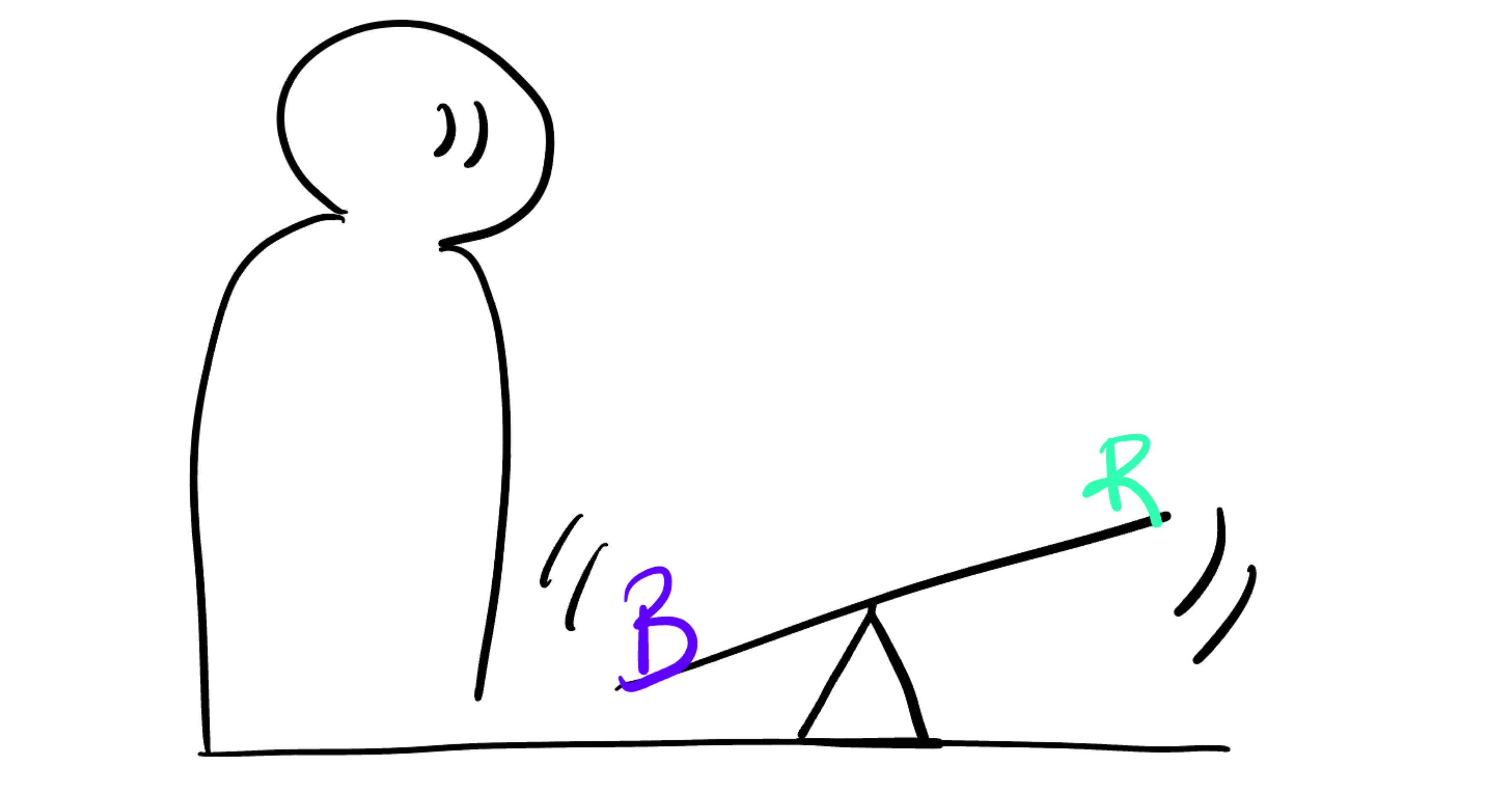
The trajectory you’ve been calling success, failure, or stagnation is loop dominance. And dominance can shift, but only if you know which loop to push.
Foundation 9 is part of Simularch’s Foundation Series, a sequential introduction to system dynamics. If you’re reading this for the first time, Foundation 0 is the place to start.
🧩 What’s Coming Next
This foundations series will build your systems thinking toolkit step by step:
2 | Stop! Let’s Talk Stocks: Not Wall Street, Just Bathtubs ✔️
3 | Go With the Flow: Pipes, Currents, and Traffic Jams (A Love Story) ✔️
4 | Causal Loop Diagrams 101: Stop Talking, Start Drawing ✔️
7 | Reinforcing Feedback Loops: Congratulations, You Made It Worse ✔️
📚 Main Resources
Meadows, D. H. (2015). Thinking in Systems. Chelsea Green Publishing.
Sterman, J.D. (2000) Business Dynamics: Systems Thinking and Modeling for a Complex World. Irwin McGraw-Hill, Boston.
My lecture notes from “System Dynamics” and “Simulation” classes :)
Some explanations and phrasings closely follow or directly quote these sources. The text was refined for coherence and citation accuracy with the assistance of large language models.