

System Dynamics | Foundation 10: One-Stock System Dynamics
Choose Your Own Catastrophe

Ask someone where a population ends up, and they will say: somewhere proportional to where it began. Something reasonable.
Structure disagrees.
The destination of a one-stock system is not a function of its starting conditions. It is a function of the ratio of its flows such as birth rates, mortality fractions, external forcing, feedback strength. Change the structure, change the destination. Push the stock harder, change nothing. The system returns to exactly where structure said it would go.
We will run one population, rabbits, through every structurally distinct condition a single stock can face. Same rabbits. Different structure. Entirely different curves.
By the end, each curve is a diagnostic. Learn the shape, read backwards to the structure.
Part I: The Stock as a Passive Counter
When flows ignore the stock completely, the population has no effect on what enters or leaves. It is a passive counter that is adding and subtracting what arrives, with no ability to push back.
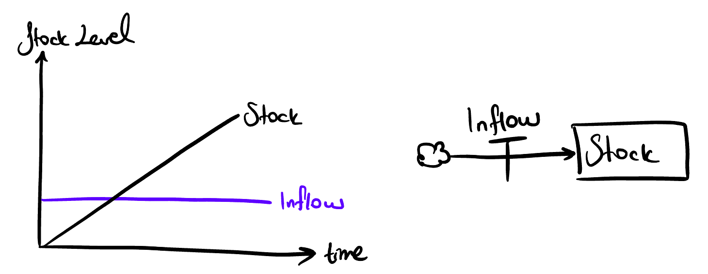
A fixed immigration program introduces the same number of rabbits each year. The population climbs at a fixed rate. Not because anything is thriving, because arithmetic says so.
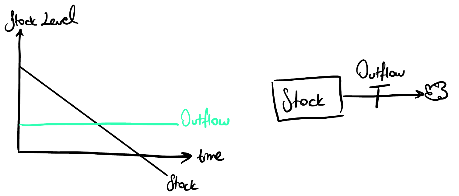
Now reverse it: a constant mortality rate, no immigration. The stock falls linearly until it hits zero (if stock represent sth else, it can go below zero). Not because anything went wrong, because the structure contains no mechanism to protect or replenish the stock.
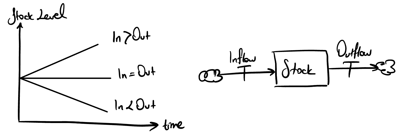
Both present: three outcomes, all arithmetic. If immigration exceeds mortality, the stock grows. If they match, it flatlines. If mortality exceeds immigration, it declines.
The core insight of this section: no feedback means no self-correction. The population cannot slow itself when it grows too fast. It cannot recover when it falls too low. It simply obeys whatever the external flows dictate.
Part II: When the Stock Drives Its Own Flows
Now add feedback. Let the flows respond to the stock’s own level.
The simplest version: the net growth rate is proportional to the current population. Twice as many rabbits produce twice as many offspring. A reinforcing loop. The flow is a linear function of the stock, but the behavior this produces over time is not linear at all.
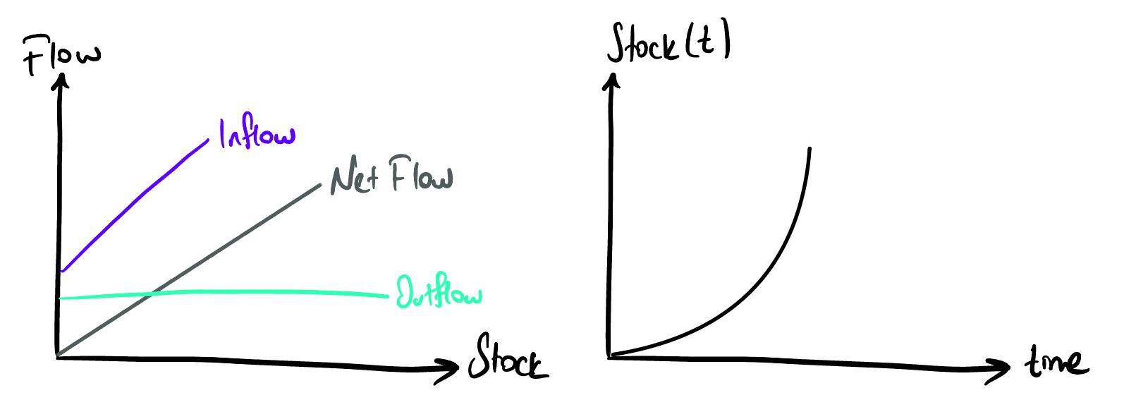
The population grows exponentially. The doubling time is constant regardless of population size, whether there are ten rabbits or ten million. The structure doubles, not any particular count. Constant doubling time is the fingerprint of pure reinforcing feedback.
Now flip the sign. Mortality proportional to current population, no immigration.
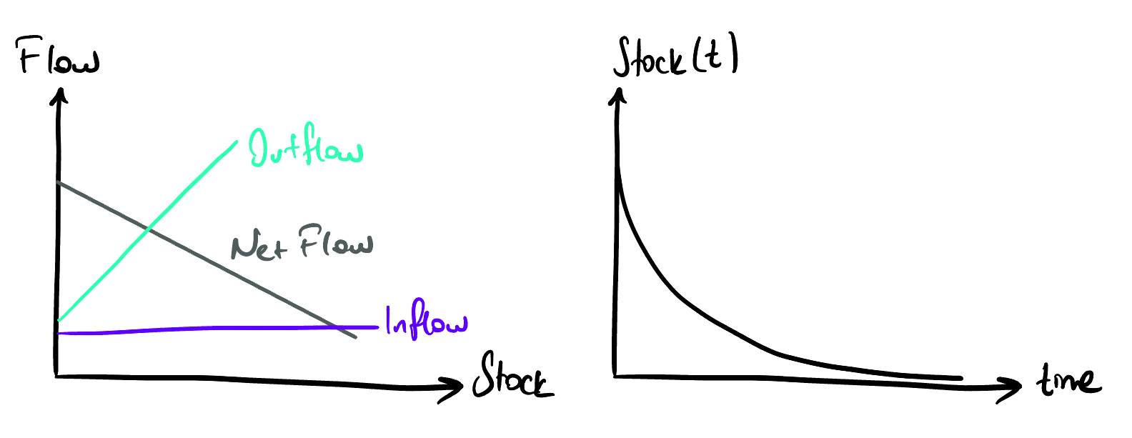
The stock decays exponentially toward zero. The larger the population, the faster it loses members in absolute terms, but the rate of loss is always proportional, so the curve decelerates as it approaches zero, never quite arriving.
Notice: this is not goal-seeking yet. There is no setpoint, no desired level the system is trying to reach. The stock simply decays because the only flow is a proportional outflow. Goal-seeking requires something to seek, a target the structure is trying to match. That comes next.
The core insight of this section: the curve is not linear, but the structure is. Linearity describes the relationship between flow and stock, not the shape of the behavior it produces. This matters because it determines everything about how the system can be analyzed and changed.
Part III: Coupling, When Structure Meets the World
Most real populations live at the intersection of feedback and external forcing. Three structural configurations. Three distinct behavioral signatures. Three distinct types of equilibrium.
Case A: Balancing Outflow + Constant Immigration
A conservation program introduces a fixed number of rabbits into a reserve each year, constant immigration. Natural mortality removes a fraction of the current population: the larger the population, the more die. This is a balancing loop on the outflow side.
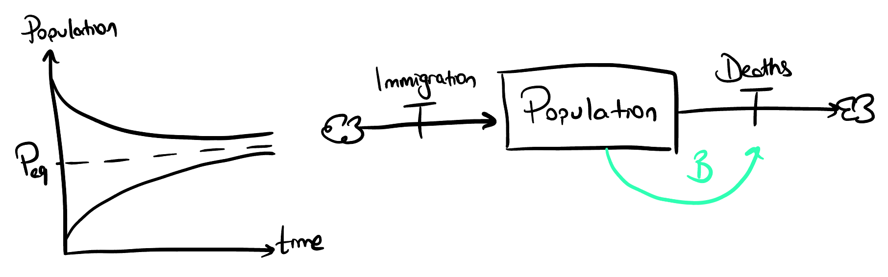
The population rises. Mortality rises with it. Eventually the two balance, and the stock stops changing. This is equilibrium: total inflow equals total outflow.
Start with ten rabbits or ten thousand, both curves arrive at the same level. This is a stable equilibrium. Disturb it and the system returns. The balancing loop corrects discrepancy from either direction.
The equilibrium level is set by the ratio of immigration rate to mortality fraction, two structural parameters. Not by the initial population.
Case B: Reinforcing Inflow + Fixed Hunting Quota
Remove the immigration program. Rabbits reproduce naturally, proportional to their population, a reinforcing loop on the inflow. But hunters take a fixed quota each season, regardless of population size.
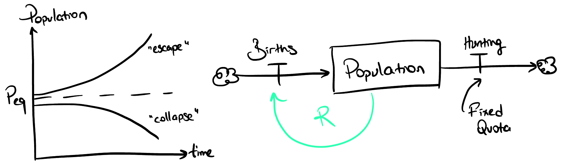
An equilibrium exists mathematically, the level at which births exactly match the fixed quota. But it is unstable. It does not attract, it repels.
Above the threshold: the reinforcing loop generates more births than the fixed quota removes. Population escapes upward. Below the threshold: the quota removes more than the reinforcing loop replaces. Population collapses toward zero. Both trajectories run away from the equilibrium line.
This is the structural anatomy of a tipping point. Not a metaphor, a feedback configuration in which a reinforcing loop faces a constant drain, and the two balance at exactly one unstable level. The equilibrium exists on paper. No real population can rest there. Cross it in either direction and the system accelerates away.
This is also why fixed quotas are structurally dangerous for populations driven by reinforcing feedback. The quota does not adjust when the population falls. The reinforcing loop weakens when the population falls. These two properties combine to make collapse self-reinforcing past a threshold that is invisible until crossed.
Case C: Balancing Inflow + Fixed Hunting Quota
Now the habitat limits reproduction. As crowding increases, birth rates fall. A balancing loop on the inflow through carrying capacity. A fixed harvest continues.
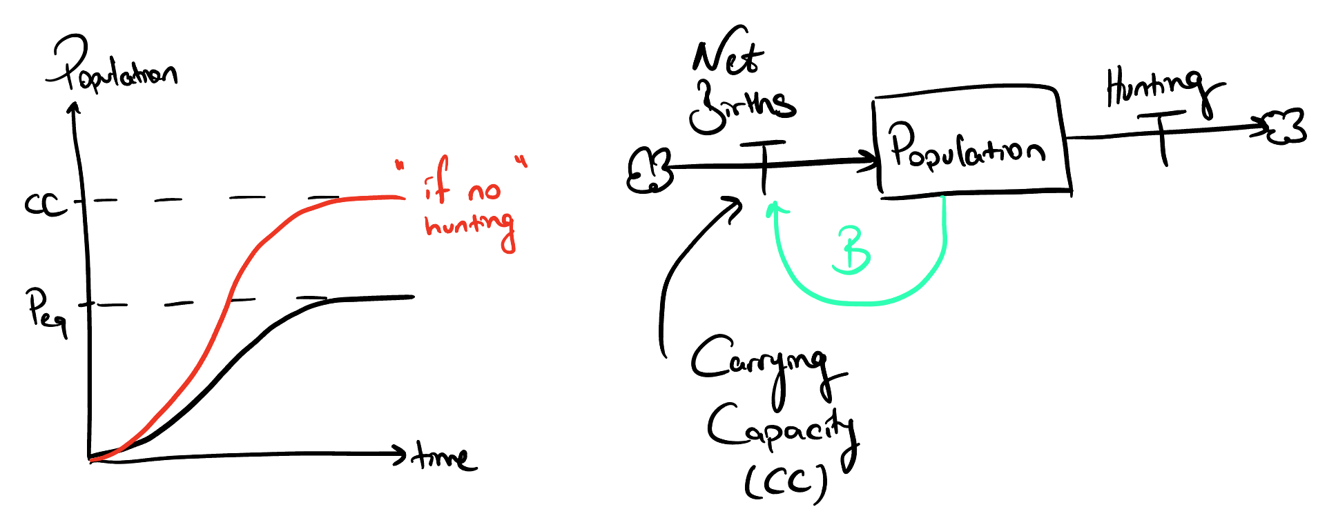
The population follows an S-shaped path, settling below the natural carrying capacity. The harvest pulls the equilibrium permanently downward.
This equilibrium is stable, the balancing loop corrects from both directions. But the system cannot reach its biological ceiling. The structural gap between carrying capacity and equilibrium is proportional to the harvest rate.
The structural implication is precise: releasing more rabbits into this structure changes nothing in the long run. The system returns to the same level. To raise the equilibrium, you must either reduce the harvest rate or increase the carrying capacity. Not more rabbits, different structure.
Part IV: Reading the Fingerprint
You now have the complete vocabulary.
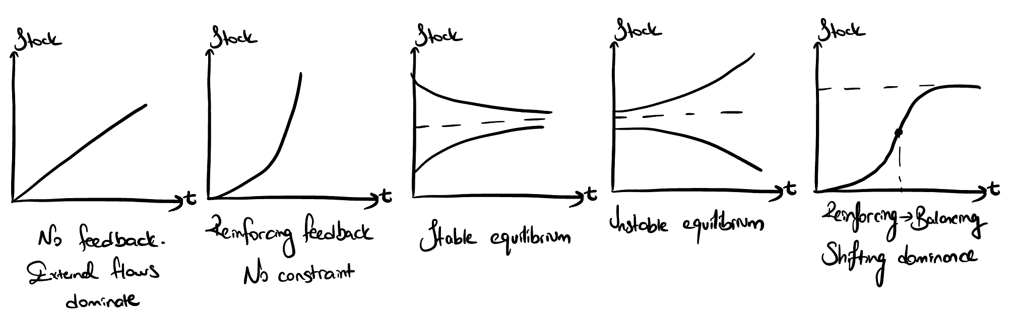
A behavior graph is not just a picture of what happened. It is a diagnostic of the structure underneath.
A straight line means no feedback, external flows dominate and the stock is a passive counter. An accelerating curve with no ceiling means a reinforcing loop is running without constraint. A decelerating curve that flattens at a ceiling means a balancing loop is dominant and external forcing is present, the system is goal-seeking to a stable equilibrium. Two curves diverging from a middle line, one escaping upward, one collapsing downward, means a reinforcing loop is fighting a constant drain, and you are looking at an unstable equilibrium, a tipping point. An S-shaped curve means reinforcing feedback dominated early and balancing feedback took over as the stock approached its ceiling, shifting dominance, which Foundation 9 covered in full.
These five shapes are the complete behavioral vocabulary of a one-stock system. Structure selects from this vocabulary. The curve you observe tells you which structure is running.
This is why behavior-over-time graphs are not decoration in system dynamics. They are the first diagnostic step. Before you draw a structure diagram, before you name a feedback loop, you look at the curve. The curve tells you where to look.
What Comes Next
Everything in this article assumes the system acts on perfect, immediate information. The population level is perceived correctly. Corrective flows respond right now. No lag between signal and action.
Real systems do not work this way.
When the hunting quota is set based on last season’s count, and that count arrives months after the season ends, and the quota decision takes more months to implement, the corrective action is steering with a delayed signal. The structure is the same. The equilibrium is the same. But the path to equilibrium warps.
Goal-seeking becomes oscillation. The population overshoots and undershoots around the level it is trying to find. In some structures, it never settles at all.
Same structure. Delayed feedback. Completely different curve.
That is Foundation 11.
🧩 What’s Coming Next
This foundations series will build your systems thinking toolkit step by step:
2 | Stop! Let’s Talk Stocks: Not Wall Street, Just Bathtubs ✔️
3 | Go With the Flow: Pipes, Currents, and Traffic Jams (A Love Story) ✔️
4 | Causal Loop Diagrams 101: Stop Talking, Start Drawing ✔️
7 | Reinforcing Feedback Loops: Congratulations, You Made It Worse ✔️
10 | One-Stock System Dynamics: Choose Your Own Catastrophe ✔️
11 | Delays: Everything Is Fine (As of Six Months Ago)
📚 Main Resources
Meadows, D. H. (2015). Thinking in Systems. Chelsea Green Publishing.
Sterman, J.D. (2000) Business Dynamics: Systems Thinking and Modeling for a Complex World. Irwin McGraw-Hill, Boston.
My lecture notes from “System Dynamics” and “Simulation” classes :)
Some explanations and phrasings closely follow or directly quote these sources. The text was refined for coherence and citation accuracy with the assistance of large language models.